Gradient Class Activation Map (Grad-CAM) Summary¶

GradCam

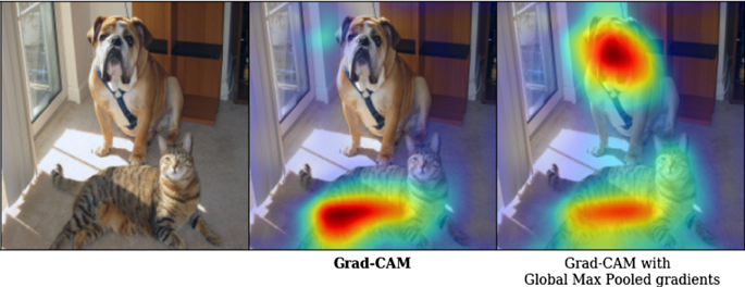
The following note demonstrates the logic procedure of how a GradCam is computed. For details, please see: Grad-CAM: Why did you say that? Visual Explanations from Deep Networks via Gradient-based Localization

Assumption¶

Class Activation Mapping¶

$y^{c} = \sum\limits_{k} w^k_c \frac{1}{Z} \sum\limits_{i} \sum\limits_{j} A^k_{ij}$

The penultimate layer produces $K$ activation map $A^K$ with width $u$ and height $v$ .

The feature goes through $\frac{1}{Z} \sum\limits_{i} \sum\limits_{j}$ , which is called global averaged pooled, and then linearly transforemd to $y^{c}$ for each class $c$ .

Procedure¶

1. Choose the penultimate layer.¶

This is the layer where we want to visualize the activation map. The reason why it is called the penultimate layer is because the last layer of a model is usually the layer computing class-specific loss (i.e. Sigmoid loss, softmax loss, etc). The penultimate layer is a layer, which is before the last layer, that we want to compute the loss respect to.

2. Compute the class-specific loss (i.e. loss of $y^{c}$ ) on the last layer of the model.¶

3. Compute the gradients of $y^c$ respect to the penultimate layer's activation map $A^K$ .¶

$\alpha^c_k = \frac{1}{Z} \sum\limits_{i} \sum\limits_{j} \frac{\partial y^c}{\partial A^k_{ij}}$

The dimension of the gradients is then reduced from (batch_size, u, v, channel)to (channel) by averaging the values in the first three axises. In the paper, this dimension reduction is called global-average-pooling.

This result denoted as $\alpha^c_k$ represents a partial linearization of the penultimate layer to the loss, which captures the importance of the activation $A^k$ for a target $c$ .

4. Elemently-wise multpile the the gradient with the Activation map.¶

5. Remove any negative results by applying the Relu function over the result.¶

Only interested in the positive influence on the class of interest. (i.e. Pixels whose intensity should increase in order to increase $y^{c}$ )

$L^c_{Grad-CAM} = Relu(\sum\limits_{k} \alpha^c_k A^k)$